
In deep learning (DL), we aim to find the optimal weights $\mathbf{W}$ and biases $\mathbf{b}$ with respect to a cost function. As the name suggests, deep neural networks consist of many layers chained together, leading to a highly complex computational graph. Since calculating the exact inverse of these chained layers is virtually impossible, we must rely on numerical optimization. AdamW has become the de-facto standard and a robust baseline for training modern DL models.
We approach understanding AdamW by looking at its evolution, starting from the Stochastic Gradient Descent (SGD) algorithm. At each step of the timeline, we aim to understand what specific problem the algorithm is solving compared to its predecessor.
| Era | Method | Core Innovation |
|---|---|---|
| 1950s | SGD | Update weights by the negative gradient. |
| 1960s | Momentum | Adds velocity to smooth out updates and overcome local minima. |
| 1980s | Nesterov | A “look-ahead” mechanism before calculating the gradient. |
| 2011 | AdaGrad | Per-parameter learning rates based on feature frequency. |
| 2012 | RMSProp | Sliding window adaptive rates (solves AdaGrad’s “stalling”). |
| 2014 | Adam | Combines Momentum, RMSProp, and Bias Correction. |
| 2017 | AdamW | Decouples weight decay from adaptive updates for better regularization. |
| 2020+ | Lion / Sophia | New experimental optimizers (Memory efficient / Second-order). |
The complete evolutionary timeline of Adam & Co.
Training Objective
The objective of training is to find the set of weights $\mathbf{W}$ and biases $\mathbf{b}$ that minimize the distance between the network output $\mathbf{o}$ and target labels $\mathbf{y}$:
\[\hat{\mathbf{W}}, \hat{\mathbf{b}} = \arg\min_{\mathbf{W}, \mathbf{b}} \frac{1}{N} \sum_{i=1}^N C(\mathbf{W}, \mathbf{b}; \mathbf{x}_i, \mathbf{y}_i) \tag{1}\]where $C$ is the cost (loss) function and $N$ is the size of the dataset.
Stochastic Gradient Descent (SGD)
SGD is the fundamental algorithm used to update learnable parameters. The gradient $\nabla C$ indicates the direction of steepest increase; thus, we move in the opposite direction:
\[\mathbf{W}_t = \mathbf{W}_{t-1} - \eta \nabla_{\mathbf{W}} C, \quad \mathbf{b}_t = \mathbf{b}_{t-1} - \eta \nabla_{\mathbf{b}} C \tag{2}\]where the hyperparameter $\eta \in \mathbb{R}^+$ is the learning rate.
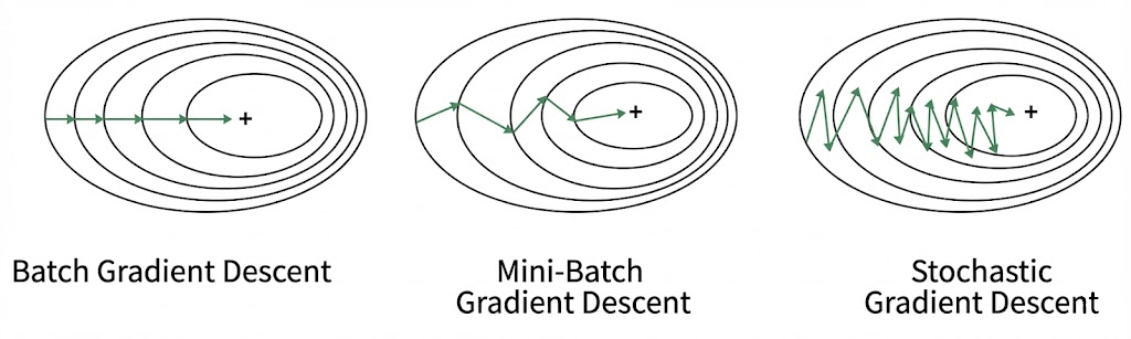
In practice, calculating the cost over the entire dataset ($N$) is computationally prohibitive. Instead, we approximate the gradient using mini-batches of size $M < N$. Selecting the optimal $M$ is a balancing act:
- Stochasticity for Generalization: Because each mini-batch is a random sample, the resulting loss surface fluctuates slightly at every step. This “noise” helps the optimizer escape sharp local minima and guides the network toward flat minima, which generally improves the model’s ability to generalize to unseen data.
- Gradient Stability: Larger mini-batches provide higher “gradient quality” by averaging out noise, leading to smoother updates. However, if $M$ is too large, the lack of stochastic pressure may cause the network to overfit or settle into poor minima.
Gradient Descent With Momentum
Momentum addresses the problem of “oscillations” in narrow valleys of the loss surface. It maintains a running average of the gradients (the first moment), building speed in directions where the gradient is consistent and canceling out noise where it flickers.
\[\mathbf{m}_t = \beta_1 \mathbf{m}_{t-1} + (1 - \beta_1) \mathbf{g}_{t} \tag{3} \label{eq:momentum}\] \[\mathbf{w}_t = \mathbf{w}_{t-1} - \eta \mathbf{m}_t \tag{4} \label{eq:momentum-update}\]where $\beta_1$ is the decay rate (usually $0.9$), and \(\mathbf{g}_t := \nabla_{\mathbf{w}} C_t\). By substituting $\eqref{eq:momentum}$ into $\eqref{eq:momentum-update}$, we can derive the alternative Polyak’s Heavy Ball formulation:
\[\mathbf{w}_{t+1} = \mathbf{w}_t - \alpha \mathbf{g}_t + \beta (\mathbf{w}_t - \mathbf{w}_{t-1}) \tag{5}\]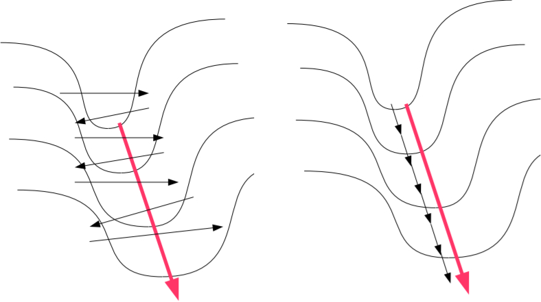
Vanilla gradient descent (left) vs. Gradient descent with momentum (right).
Nesterov Accelerated Gradient (NAG)
NAG is a “look-ahead” modification to momentum. The core problem with standard Polyak’s momentum is that it is “blind” to the future: it calculates the gradient at the current position, adds the accumulated velocity, and effectively “hopes” it doesn’t overshoot. In high-curvature valleys, this often leads to the algorithm flinging itself up the opposite slope before it can react.
NAG solves this by being proactive. It calculates the gradient at the point where the momentum would take you, allowing the optimizer to anticipate the landscape and apply a “braking” force if it’s about to overshoot.
\[\mathbf{v}_t = \gamma \mathbf{v}_{t-1} + \eta \nabla C(\mathbf{w}_{t-1} - \gamma \mathbf{v}_{t-1}) \tag{6}\] \[\mathbf{w}_t = \mathbf{w}_{t-1} - \mathbf{v}_t \tag{7}\]In deep learning libraries like PyTorch, this is often rearranged to avoid calculating gradients at a “virtual” point:
\[\mathbf{v}_t = \gamma \mathbf{v}_{t-1} + \mathbf{g}_t \tag{8}\] \[\mathbf{w}_t = \mathbf{w}_{t-1} - \eta (\mathbf{g}_t + \gamma \mathbf{v}_t) \tag{9}\]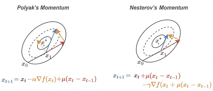
Polyak vs. Nesterov: Polyak calculates the gradient (orange) before the velocity jump (red); Nesterov calculates it after the jump.
Adaptive Gradient (AdaGrad)
AdaGrad adjusts the learning rate for each parameter individually. It gives smaller updates to frequent features and larger updates to infrequent (sparse) ones by accumulating past squared gradients.
\[G_t = G_{t-1} + \mathbf{g}_t^2 \tag{10}\] \[\mathbf{w}_{t+1} = \mathbf{w}_t - \frac{\eta}{\sqrt{G_t + \epsilon}} \odot \mathbf{g}_t \tag{11}\]The primary concern is that $G_t$ grows monotonically. Eventually, the effective learning rate shrinks toward zero, causing training to stall—a phenomenon known as the “Death of AdaGrad.”
Root Mean Square Propagation (RMSProp)
RMSProp fixes AdaGrad by replacing the raw sum with an exponentially decaying moving average. This allows the optimizer to “forget” the distant past and maintain a productive learning rate throughout training.
\[E[\mathbf{g}^2]_t = \rho E[\mathbf{g}^2]_{t-1} + (1 - \rho) \mathbf{g}_t^2 \tag{12}\] \[\mathbf{w}_{t+1} = \mathbf{w}_t - \frac{\eta}{\sqrt{E[\mathbf{g}^2]_t + \epsilon}} \odot \mathbf{g}_t \tag{13}\]Adaptive Moment Estimation (Adam)
Adam is the fusion of Momentum and RMSProp. It tracks both the First Moment ($\mathbf{m}_t$, the mean) and the Second Moment ($\mathbf{v}_t$, the uncentered variance).
Update Moments:
\[\mathbf{m}_t = \beta_1 \mathbf{m}_{t-1} + (1 - \beta_1) \mathbf{g}_t \tag{14}\] \[\mathbf{v}_t = \beta_2 \mathbf{v}_{t-1} + (1 - \beta_2) \mathbf{g}_t^2 \tag{15}\]Bias Correction: Since $\mathbf{m}_t$ and $\mathbf{v}_t$ are initialized at zero, they are biased toward zero in early steps. We correct this:
\[\hat{\mathbf{m}}_t = \frac{\mathbf{m}_t}{1 - \beta_1^t}, \quad \hat{\mathbf{v}}_t = \frac{\mathbf{v}_t}{1 - \beta_2^t} \tag{16} \label{eq:adam-bias-correction}\]Update Weights:
\[\mathbf{w}_{t+1} = \mathbf{w}_t - \frac{\eta}{\sqrt{\hat{\mathbf{v}}_t} + \epsilon} \hat{\mathbf{m}}_t \tag{17}\]Adam effectively combined three critical ideas. It uses $\hat{\mathbf{m}}_t$ to navigate high-curvature valleys, $\hat{\mathbf{v}}_t$ to handle non-stationary objectives, and the Bias Correction steps in Eq. $\eqref{eq:adam-bias-correction}$ to ensure the optimizer is effective from the very first iterations.
Adam with Decoupled Weight Decay (AdamW)
Despite its success, Adam had a mathematical flaw in how it handled weight decay. In standard Adam, the $L_2$ penalty is added to the gradient, meaning it also gets scaled by the inverse of $\sqrt{\mathbf{v}_t}$. This results in non-uniform regularization. AdamW decouples weight decay by applying it directly to the weights:
\[\mathbf{w}_{t+1} = \mathbf{w}_t - \underbrace{\eta \left( \frac{\hat{\mathbf{m}}_t}{\sqrt{\hat{\mathbf{v}_t}} + \epsilon} \right)}_{\text{Adaptive Update}} - \underbrace{\eta \lambda \mathbf{w}_t}_{\text{Decoupled Decay}} \tag{18}\]Beyond AdamW
Several newer optimizers address AdamW’s memory overhead and its ignorance of “curvature” (second-order information).
EvoLved SIgn Momentum (Lion)
Lion (2023) is more memory-efficient as it only tracks the sign of the momentum. It discards the second moment ($\mathbf{v}_t$), saving 50% of the optimizer memory.
\[\mathbf{w}_{t+1} = \mathbf{w}_t - \eta \cdot \text{sign}(\beta_1 \mathbf{m}_{t-1} + (1-\beta_1)\mathbf{g}_t) \tag{19}\]Second-order Stochastic Optimization (Sophia)
Sophia (2023) is a second-order optimizer designed for LLMs. It estimates the Hessian (curvature). By knowing where the landscape is flat or sharp, Sophia can take larger steps in flat directions, potentially training GPT-style models 2× faster than AdamW.
Momentum Update on Orthogonalized Nanoscale (Muon)
A newer entrant that ensures weight updates are “orthonormal.” It has shown significant efficiency in training Small Language Models (SLMs) and Mixtures of Experts (MoE) by ensuring the internal geometry of the weights remains well-conditioned.
Conclusion
The journey from SGD to AdamW represents a transition from simple gradient-following to sophisticated, per-parameter adaptive systems. AdamW remains the industry standard because it strikes a perfect balance: it is computationally efficient, handles sparse gradients well, and provides robust regularization through decoupled weight decay. While newer optimizers like Lion and Sophia offer exciting improvements in memory and convergence speed, AdamW’s reliability across diverse architectures makes it the most essential tool in the modern practitioner’s toolkit.
References
- Mitliagkas, I. Nesterov’s Momentum, Stochastic Gradient Descent. IFT 6085 - Lecture 6, 2019.
- Duchi, J., Hazan, E., & Singer, Y. Adaptive Subgradient Methods for Online Learning and Stochastic Optimization. Journal of Machine Learning Research, 2011.
- Kingma, D. P., & Ba, J. Adam: A Method for Stochastic Optimization. ICLR, 2015.
- Loshchilov, I., & Hutter, F. Decoupled Weight Decay Regularization. ICLR, 2019.
- Chen, X., et al. Symbolic Discovery of Optimization Algorithms. arXiv preprint arXiv:2302.06675, 2023. (Lion)
- Liu, H., et al. Sophia: A Scalable Stochastic Second-order Optimizer for Language Model Pre-training. arXiv preprint arXiv:2305.14342, 2023.
- Keller, J., et al. Muon: Momentum Update on Orthogonalized Nanoscale. 2024.