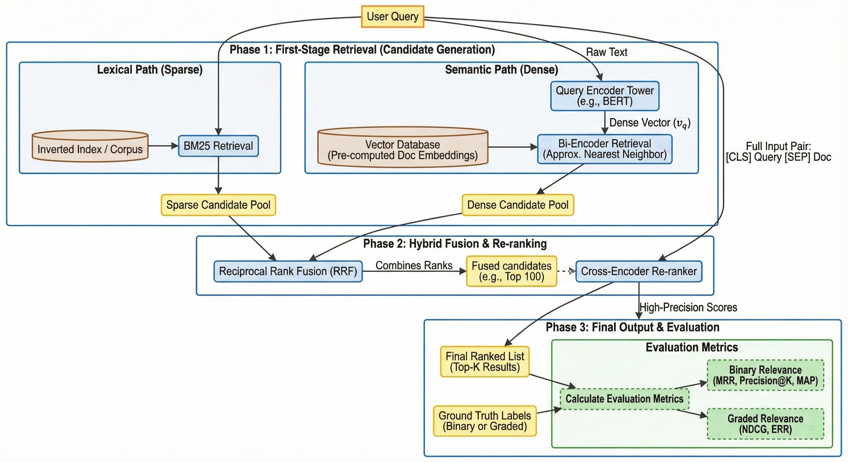
Modern information retrieval (IR) systems face a fundamental trade-off between computational efficiency and ranking precision. In a world where corpora consist of billions of documents, it is impossible to apply complex, query-aware neural models to every document in real-time. To solve this, the industry has standardized the Multi-stage Ranking Pipeline.
This architecture functions like a funnel: the initial stages use lightweight, high-recall methods to filter the corpus down to a few hundred candidates, while subsequent stages use increasingly sophisticated models to refine the order of those candidates for maximum relevance.
First stage retrieval
The first stage of the pipeline is often referred to as “Candidate Generation.” Its primary objective is high recall—ensuring that as many relevant documents as possible are caught in the “net,” even if many irrelevant ones are included. Because this stage must scan the entire corpus (millions or billions of documents), it must be extremely fast and typically relies on pre-computed indices.
Lexical / Sparse Retrieval
In the first and coarse stage, documents are retrieved based on exact keywords (lexical matching). The query is represented as a large sparse vector (most entries are 0) and the mapping is based on vocabulary (bag of words). This retrieval is the cheapest but also most inaccurate as it fails to capture the underlying intent or synonyms.
Term Frequency-Inverse Document Frequency (TF-IDF)
The overall formula is the product of two separate components:
\[\text{TF-IDF}(q, d, D) = \text{TF}(q, d) \times \text{IDF}(q, D) \tag{1}\]- $q \in Q$: term of query
- $d \in D$: document
- $D$: all documents (corpus)
Term Frequency (TF)
This measures how frequently a term $q$ appears in a specific document $d$. The most common way to calculate it (normalized to document length) is:
\[\text{TF}(q, d) = \frac{f_{q, d}}{\sum_{q' \in d} f_{q', d}}\]- $f_{q, d}$: The number of times term $q$ appears in document $d$.
- Denominator: The total number of terms in document $d$.
Inverse Document Frequency (IDF)
This measures how important a term is across the entire collection of documents $D$. It reduces the weight of terms that appear very frequently (like “the” or “is”) and increases the weight of terms that are rare.
\[\text{IDF}(q, D) = \log \left( \frac{N}{|\{d \in D : q \in d\}|} \right) \in \left[0, \infty \right) \tag{2}\]- $N = \lvert D\rvert$: Total number of documents in the corpus.
- $\lvert{d \in D : q \in d}\rvert$: Number of documents where the term $q$ appears (Document Frequency).
The rarer a term in the corpus is, the larger the IDF will be.
The Aggregated Formula
If your query $Q$ consists of terms ${q_1, q_2, \dots, q_n}$, the document score is:
\[\text{score}(d, D, Q) = \sum_{q_i \in Q} \text{TF-IDF}(q_i, d, D) \tag{3}\]While TF-IDF was a revolutionary starting point for search, it has two major “blind spots” that make it less effective for modern information retrieval.
- Its linear scaling fails to account for term frequency saturation, allowing repetitive “keyword stuffing” to disproportionately and inaccurately inflate a document’s relevance score.
- Its lack of adaptive normalization creates a bias that unfairly penalizes long, comprehensive content or over-rewards short documents with accidental keyword matches.
Best Matching 25 (BM25)
BM25 is the state-of-the-art lexical ranking function. For a query $Q$ containing terms $q_1, q_2, \dots, q_n$, the score for document $d$ is:
\[\text{score}(d, D, Q) = \sum_{q \in Q} \text{IDF}(q, D) \cdot \frac{f_{q, d} \cdot (k_1 + 1)}{f_{q, d} + k_1 \cdot \left(1 - b + b \cdot \frac{|d|}{\text{avgdl}}\right)} \tag{4}\]- Term Frequency $f_{q, d}$: How many times the query term $q$ appears in document $d$.
- Average Doc Length $\text{avgdl}=\frac{1}{\lvert D \rvert}\sum_{d \in D}\lvert d \rvert$: The average number of words across all documents in the collection.
- Saturation Constant $k_1$: Controls how quickly the “reward” for a repeating word plateaus (usually $1.2$ to $2.0$).
- Length Penalty $b$: Controls how much document length affects the score (usually $0.75$).
The BM25 version of IDF
It is important to note that BM25 uses a slightly modified version of Inverse Document Frequency (IDF) compared to standard TF-IDF to ensure the math remains robust for very common words:
\[\text{IDF}(q, D) = \log \left( \frac{N - n(q, D) + 0.5}{n(q, D) + 0.5} + 1 \right) \tag{5}\]- $N = \lvert D\rvert$: Total number of documents in the collection.
- $n(q, D) = \lvert{d \in D : q \in d}\rvert$: Number of documents that contain the term $q$.
Fostering understanding for the BM25 formula
The BM25 formula seems quite complicated at first glance. To understand it better, let’s define
\[g(q, d) = \frac{f_{q, d} \cdot (k_1 + 1)}{f_{q, d} + k_1 \cdot \left(1 - b + b \cdot \frac{|d|}{\text{avgdl}}\right)} \tag{6}\]and look at some edge cases:
\[\lim_{f_{q, d} \to \infty} g(q, d) = k_1 + 1 \tag{7} \label{eq:large-f}\] \[g(q, d) |_{k_1 = 0} = 1 \tag{8} \label{eq:small-k1}\] \[\lim_{k_1 \to \infty} g(q, d) = \frac{f_{q, d}}{1 - b \left(\frac{|d|}{\text{avgdl}} - 1\right)} \tag{9} \label{eq:large-k1}\] \[g(q, d)|_{\lvert d \rvert = \text{avgdl}\ \lor\ b=0} = \frac{f_{q, d} \cdot (k_1 + 1)}{f_{q, d} + k_1} \tag{10} \label{eq:small-document-penalty}\] \[\lim_{\lvert d \rvert \to \infty}g(q, d) = \lim_{b \to \infty} g(q, d) = 0 \tag{11} \label{eq:large-document-penalty}\] \[\lim_{k_1 \to \infty} g(q, d)|_{\lvert d \rvert = \text{avgdl}} = f_{q, d} \tag{12} \label{eq:large-k1-and-avg-length}\]As can be easily seen in $\eqref{eq:large-f}$ a large term frequency asymptotes $g$ to the constant $k_1 + 1$, effectively limiting the keyword stuffing. While as can be seen in $\eqref{eq:small-k1}$ a small $k_1$ pushes the metric to disregard term frequency. A large $k_1$ on the contrary, as can be seen in $\eqref{eq:large-k1}$ and $ \eqref{eq:large-k1-and-avg-length}$ reduces the fraction to the Term Frequency divided by the Term Frequency plus the length penalty term. As can be easily seen in $\eqref{eq:small-document-penalty}$ and $\eqref{eq:large-document-penalty}$ a larger $b$ puts a stronger penalty on large document lengths.
Semantic / Dense Retrieval
The semantic or dense methods use deep learning (like BERT) to map text into a mathematical space where similar meanings are physically close together. Key Advantage: They solve the vocabulary gap. They “know” that “dog” and “canine” are related, even if they share no letters.
Two-Tower Encoders (Bi-Encoders)
Two-Tower Architecture: It uses two separate “towers” (neural networks). One tower processes the query, and the other processes the document. They never “see” each other during the encoding phase. Once both the query and the document have been turned into vectors ($v_q$ and $v_d$), their relevance is calculated using simple vector geometry, usually Cosine Similarity or Dot Product:
\[\text{score}(q, d) = \frac{v_q \cdot v_d}{\|v_q\| \|v_d\|} = \cos(\theta) \tag{13}\]The most critical advantage of Bi-Encoders over other neural methods (like Cross-Encoders) is efficiency at scale:
- Offline Encoding: Document vectors are stored in a Vector Database like Pinecone.
- Real-time Retrieval: You only need to encode the query (one tower pass).
- Speed: Vector comparison (Dot Product) is extremely fast on modern hardware.
Scaling Search with ANN Indices
Calculating exact Cosine Similarity against millions of vectors is too slow for real-time applications. Instead, vector databases use Approximate Nearest Neighbor (ANN) algorithms to speed up the process:
- Hierarchical Navigable Small Worlds (HNSW): Constructs a multi-layered graph that allows the search to “skip” through clusters of data to find the neighborhood of the query vector quickly. It provides high accuracy and sub-millisecond latency at the cost of high RAM usage.
- Inverted File with Product Quantization (IVF-PQ): Partitions the vector space into Voronoi cells (IVF) and compresses the vectors using Product Quantization (PQ). This allows billions of documents to fit in memory, though at a slight cost to precision compared to HNSW.
Hybrid Search
Most production systems today use Hybrid Search, which combines both lexical (BM25) and semantic (Bi-Encoder) retrieval to ensure both precision for exact terms and recall for conceptual intent.
Reciprocal Rank Fusion (RRF)
To combine systems with different score scales (e.g., BM25 vs Cosine Similarity), we use RRF:
\[\text{RRFscore}(d \in D) = \sum_{r \in R} \frac{1}{k + \text{rank}(r, d)} \tag{14}\]- $R$: The set of rankers.
- $\text{rank}(r, d)$: The position of document $d$ in the results of ranker $r$ (starting at 1).
- $k$: A smoothing constant (typically set to 60).
Refining / Re-ranking
Once we have a narrowed-down pool of candidates (e.g., Top 100) from our hybrid search, we pass them to the Cross-Encoder for the final, most precise ranking.
Cross-Encoder
Unlike the Bi-Encoder, the Cross-Encoder processes the query and document simultaneously.
- Input:
[CLS] Query Text [SEP] Document Text. - Full Self-Attention: Every word in the query can “attend” to every word in the document.
- Output: A single probability score representing relevance.
Evaluation Metrics
Evaluation is the cornerstone of IR research. Without robust metrics, it is impossible to determine if a pipeline change represents a true improvement. We categorize these metrics based on the nature of the “Ground Truth” labels provided by human annotators.
Binary Relevance
In binary evaluation, a document is either relevant (1) or non-relevant (0). This is most common in navigational search or simple question-answering tasks where there is a clear “hit” or “miss.”
Mean Reciprocal Rank (MRR)
MRR only cares about the rank of the very first relevant item.
\[\text{RR} = \frac{1}{\text{rank of 1st relevant item}} \tag{15}\]Precision@K
Proportion of relevant documents in the top $K$.
\[P_K = \frac{T_{P,K}}{K} \tag{16}\]Average Precision (AP)
AP considers the entire ranking by averaging precision at every position where a relevant document is found:
\[AP = \frac{\sum_{k=1}^{n} (P@k \cdot \text{rel}_k)}{\text{Total Relevant Documents}} \tag{17}\]Mean Average Precision (MAP)
Average of $AP$ over all queries:
\[MAP = \frac{\sum_{q\in Q}AP(q)}{\lvert Q \rvert} \tag{18}\]Graded Relevance
Graded relevance recognizes that not all “hits” are equal. A “Highly Relevant” document (e.g., Grade 3) is more valuable than a “Fair” one (Grade 1). This is the standard for modern web search (e.g., Google’s 5-star rating system).
Normalized Discounted Cumulative Gain (NDCG)
NDCG is the most popular graded metric because it handles both position and varying query difficulty through normalization.
Cumulative Gain (CG)
\[CG_K = \sum_{i=1}^K rel_i \tag{19}\]Discounted Cumulative Gain (DCG)
To account for the “diminishing returns” of documents further down the list, we apply a logarithmic discount:
\[DCG_K = \sum_{i=1}^K \frac{2^{rel_i} - 1}{\log_2(i + 1)} \tag{20}\]Normalized DCG (NDCG)
We divide the actual DCG by the Ideal DCG (IDCG), which is the score of a perfect ranking.
\[NDCG = \frac{DCG}{IDCG} \tag{21}\]Expected Reciprocal Rank (ERR)
ERR models the user as a “cascade,” assuming they stop as soon as they are satisfied.
\[ERR = \sum_{r=1}^{n} \frac{1}{r} R_r \prod_{i=1}^{r-1} (1 - R_i) \tag{22}\]Where the satisfaction probability is:
\[R_i = \frac{2^{rel_i} - 1}{2^{\max(rel)}} \tag{23}\]Conclusion
The multi-stage ranking pipeline is a sophisticated orchestration of speed and intelligence. By leveraging efficient lexical and semantic retrievers to create a candidate pool, and using deep neural re-rankers to refine that pool, IR systems can serve high-quality results in milliseconds. However, the choice of evaluation metric remains the most critical decision in system design; whether one chooses MAP for comprehensive recall or NDCG for nuanced ranking significantly shifts the optimization goals of the entire pipeline.
References
- Manning, C. D., Raghavan, P., & Schütze, H. (2008). Introduction to Information Retrieval. Cambridge University Press.
- Järvelin, K., & Kekäläinen, J. (2002). Cumulated gain-based evaluation of IR techniques. ACM Transactions on Information Systems (TOIS), 20(4), 422-446.
- Robertson, S., & Zaragoza, H. (2009). The probabilistic relevance framework: BM25 and beyond. Foundations and Trends in Information Retrieval, 3(4), 333-389.
- Malkov, Y. A., & Yashunin, D. A. (2018). Efficient and robust approximate nearest neighbor search using HNSW graphs. IEEE transactions on pattern analysis and machine intelligence.
- Jegou, H., Douze, M., & Schmid, C. (2010). Product quantization for nearest neighbor search. IEEE transactions on pattern analysis and machine intelligence.
- Cormack, G. V., Clarke, C. L., & Buettcher, S. (2009). Reciprocal rank fusion outperforms data fusion and learning to rank methods. Proceedings of the 32nd international ACM SIGIR conference.
- Chapelle, O., Metlzer, D., Zhang, Y., & Grinspan, P. (2009). Expected reciprocal rank for graded relevance. Proceedings of the 18th ACM conference on Information and knowledge management (CIKM).