In the domain of efficient deep learning inference, the trade-off between model size and accuracy is usually managed through two primary compression techniques: pruning (inducing sparsity by removing weights) and quantization (reducing the bit-width of weights and activations). While both have extensive literature, a direct, rigorous comparison between the two under identical constraints has been historically sparse.
A recent paper from Qualcomm AI Research, Pruning vs Quantization: Which is Better?, provides a comprehensive analytical and empirical answer to this debate. By evaluating statistical distributions, lower-bound errors in Post-Training Quantization (PTQ), and fine-tuning dynamics in Quantization-Aware Training (QAT), the research concludes that quantization generally yields superior accuracy per bit of compression compared to unstructured pruning.
Preliminaries
The study assumes FP16 as the basic data type and measures compression gains with respect to it. Using FP16 for inference generally does not lead to a loss in accuracy. To insure a fair comparison, 50% pruning sparsity is compared to INT8 quantization, 75% sparsity to INT4 quantization, and so forth.
Quantization
The quantization experiments use symmetric uniform quantization. The quantization operation rounding-to-nearest $\mathcal{Q}(\mathbf{W})$ is defined as:
\[\mathcal{Q}(\mathbf{W})_{i, j} = s q^*,\quad q^* = \underset{q \in Q}{\arg \min} |W_{i, j} − s q|,\quad Q \in \left\{ −2^{b-1}, \dots, 2^{b − 1} - 1 \right\},\]where $s$ is the scale factor and $b$ is the bit-width.
Pruning
For pruning, the study considers magnitude pruning, which sets values closest to zero to actual zero. The pruning function $\mathcal P(\mathbf W)$ is defined as:
\[\mathcal{P}(\mathbf{W})_{i, j} = \begin{cases} W_{i, j} & \text{if } |W_{i, j}| \ge \tau \\ 0 & \text{if } |W_{i, j}| < \tau \end{cases},\quad \tau \in \mathbb R^+.\]where $\tau$ is the threshold value. Crucially, to ensure exact compression ratios for comparison, the threshold is derived from the Cumulative Distribution Function (CDF). For a target compression ratio $c \in (0,1)$ and a symmetric zero-mean distribution, the threshold satisfies:
\[\tau =F_{W}^{-1}\left(\frac{1}{2}+\frac{c}{2}\right)\]where $F^{-1}(p)$ is the inverse CDF.
Theoretical Analysis: Signal-to-Noise Ratio and Kurtosis
The authors utilize Signal-to-Noise Ratio ($\mathrm{SNR}_{dB}$) in log scale as the primary metric to compare the expected error of both methods.
\[\mathrm{SNR}_{dB}=10 \log_{10}\left(\frac{\mathbb{E}[\mathbf W^{2}]}{\mathbb{E}[(\mathbf W-\mathcal F(\mathbf W))^{2}]}\right)\]where $\mathcal F(\mathbf W)$ is the quantization or pruning function.
When analyzing a standard normal distribution—a common proxy for neural network weights—quantization significantly outperforms pruning. For example, INT4 quantization achieves an SNR of 19.1 dB, whereas 75% pruning (equivalent compression) achieves only 5.6 dB. The error in quantization is bounded and oscillates between grid nodes, while pruning introduces large errors by rounding weights to zero.
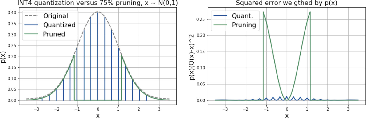
Standard Normal Comparison. (Left) Distributions after INT4 quantization vs. 75% pruning. (Right) Probability-weighted squared error.
The Exception: Heavy Tails
The study identifies a specific regime where pruning is superior: distributions with high kurtosis (heavy tails). Using a truncated Student’s t-distribution to simulate outliers, the authors found that pruning becomes beneficial only at very high compression ratios (equivalent to 2-3 bits per value) or when the data exhibits extreme outliers. However, for standard bit-widths and typical weight distributions found in the PyTorch model zoo, quantization maintains a higher SNR.
The distribution’s kurtosis was used as a predictive metric, given by:
\[\mathrm{Kurt}[X]=\frac{\mathbb{E}[(X-\mu)^{4}]}{(\mathbb{E}[(X-\mu)^{2}])^{2}}\]where $\mu$ is the mean.
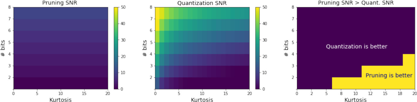
Pruning vs. Quantization error (Student's $t$). Pruning error is invariant to outlier magnitude (left), while quantization SNR degrades significantly as kurtosis increases (middle), defining the trade-off regions between the two (right).
Post-Training: Optimization and Lower Bounds
To remove algorithmic bias (e.g., comparing a poor pruning heuristic against a state-of-the-art quantization algorithm), the authors compared the methods using theoretical lower bounds on the Mean Squared Error (MSE) of layer outputs.
- Heuristic: A standard greedy algorithm provides a realizable solution (an upper bound on the error).
- Relaxation: By relaxing the integer constraints and using Semi-Definite Programming (SDP) for quantization, or Branch-and-Bound for pruning, they find the global minimum error (or a tight lower bound).
When converted to SNR for visualization, this creates a “range” of performance.
Quantization Formulation
For quantization, the problem is formulated as a mixed-integer quadratic program. The authors relax the integer constraint to $w_{i}(w_{i}-1)\ge0$ and solve the dual problem using an SDP solver to obtain a tight lower bound on the error.
Pruning Formulation
For pruning, the authors introduce a sparsity mask $m \in \mathbb{R}^n$ to formulate the optimization exactly for moderate dimensionalities.
\[E(\mathbf{w})=\min_{\mathbf{\hat{w}},\mathbf{m}}||\mathbf{X}(\mathbf{m}\odot \mathbf{\hat{w}})-\mathbf{X}\mathbf{w}_{orig}||_{2}^{2}\] \[\text{s.t.} \quad ||\mathbf{m}||_1 = k, \quad -\mathbf{m}\odot l\le \mathbf{\hat{w}}\le \mathbf{m}\odot u, \quad \mathbf{m}_{i}\in\{0,1\}, \quad l, u \in \mathbb R^+\]where $k$ is the number of non-zero elements and $\odot$ is the element-wise product. This is solved using the Branch-and-Bound method.
The results across 10 distinct layers (from MobileNet-V2, ResNet-18, and ViT) confirmed that in a post-training setting, quantization provably outperforms pruning for moderate compression ratios.
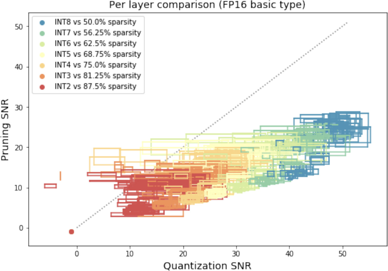
Post-Training Pruning vs. Quantization. Boxes show performance bounds across 4 models and 7 bit-widths per layer.
Fine-Tuning: QAT vs. Magnitude Pruning
The study extended the comparison to full-model fine-tuning, comparing Quantization-Aware Training (QAT) using the Learned Step Size Quantization (LSQ) method against Magnitude Pruning with gradual sparsity increases. The benchmarks included ResNet, MobileNet, EfficientNet, and ViT on ImageNet, as well as DeepLab-V3 and EfficientDet.
Key Findings
- Accuracy: At equal compression rates, pruning almost never outperformed quantization. For instance, a ResNet-50 quantized to 4-bits retained 76.3% accuracy, while the equivalently pruned model dropped to 76.1%.
- Representation Learning: By analyzing log-scale SNR and Central Kernel Alignment (CKA) distances, the authors observed that fine-tuning after pruning tends to recover the original model’s representations. In contrast, QAT leads to the learning of completely new representations.
Hardware Implications
While the paper focuses on accuracy, it notes critical hardware distinctions that further favor quantization:
- Storage Overhead: Unstructured pruning requires storing a sparsity mask (at least 1 bit per weight), adding a minimum 6.25% overhead to 16-bit weights. Quantization has negligible metadata overhead.
- Compute Efficiency: Quantization offers quadratic improvements in compute performance (e.g., INT4 vs. INT8). Conversely, unstructured pruning imposes a binary choice: either decompress weights to a dense format (wasting compute on zeros) or use dedicated hardware to skip zeros. The latter often incurs overheads that negate theoretical gains.
Conclusion
The findings suggest that for the majority of deep learning applications, quantization should be the primary strategy for model compression. Pruning appears viable primarily in scenarios necessitating extreme compression (sub-3-bit) or for distributions with exceptionally high kurtosis. The authors recommend quantizing neural networks when efficiency is required before pruning is explored.
References
Kuzmin, Andrey, et al. “Pruning vs quantization: Which is better?.” Advances in neural information processing systems 36 (2023): 62414-62427.