The “magic” behind the modern deep learning revolution isn’t just the architectures themselves, but our ability to train them efficiently. At the heart of this efficiency lies backpropagation, an algorithm that is often misunderstood as a “black box.” In reality, it is an elegant application of the Multivariate Chain Rule, implemented via Dynamic Programming. This post aims to demystify the algorithm by bridging the gap between classical textbook notations and the high-performance implementation strategies used in frameworks like PyTorch and TensorFlow.
Notations
In the following, we introduce the notations representing the computations within a neural network. As we progress from simple neurons to complex graphs, the notation evolves to remain intuitive.
Textbook Notation
At its most fundamental level, a neuron consists of a linear transformation followed by a non-linear activation function:
\[f: \mathbb{R}^n \to \mathbb{R}, \quad f(\mathbf{x}) = \sigma(\mathbf{w}^\top \mathbf{x} + b) \tag{1}\]where $\sigma: \mathbb{R} \to \mathbb{R}$ is the activation function, $\mathbf{w} \in \mathbb{R}^n$ is the weight vector, and $b \in \mathbb{R}$ is the scalar bias. For multiple neurons operating on the same input, we use matrix notation:
\[f: \mathbb{R}^n \to \mathbb{R}^m, \quad f(\mathbf{x}) = \sigma(\mathbf{W}\mathbf{x} + \mathbf{b}) \tag{2} \label{eq:multi-neurons}\]where $\mathbf{W} \in \mathbb{R}^{m \times n}$ is the weight matrix and $\mathbf{b} \in \mathbb{R}^m$ is the bias vector. We can think of the rows of the weight matrix $\mathbf{w}_i$ and the $i$-th element of the bias $b_i$ as belonging to the $i$-th neuron.
We define this operation as a layer $l$:
\[\mathbf{a}^l = \sigma(\mathbf{W}^l \mathbf{a}^{l-1} + \mathbf{b}^l), \quad l \in \{1, \dots, L\} \tag{3}\]In a Fully Connected Neural Network (FCNN), we chain these layers together:
\[\mathbf{o} = f_L(f_{L-1}(\dots f_1(\mathbf{x}) \dots)) \tag{4}\]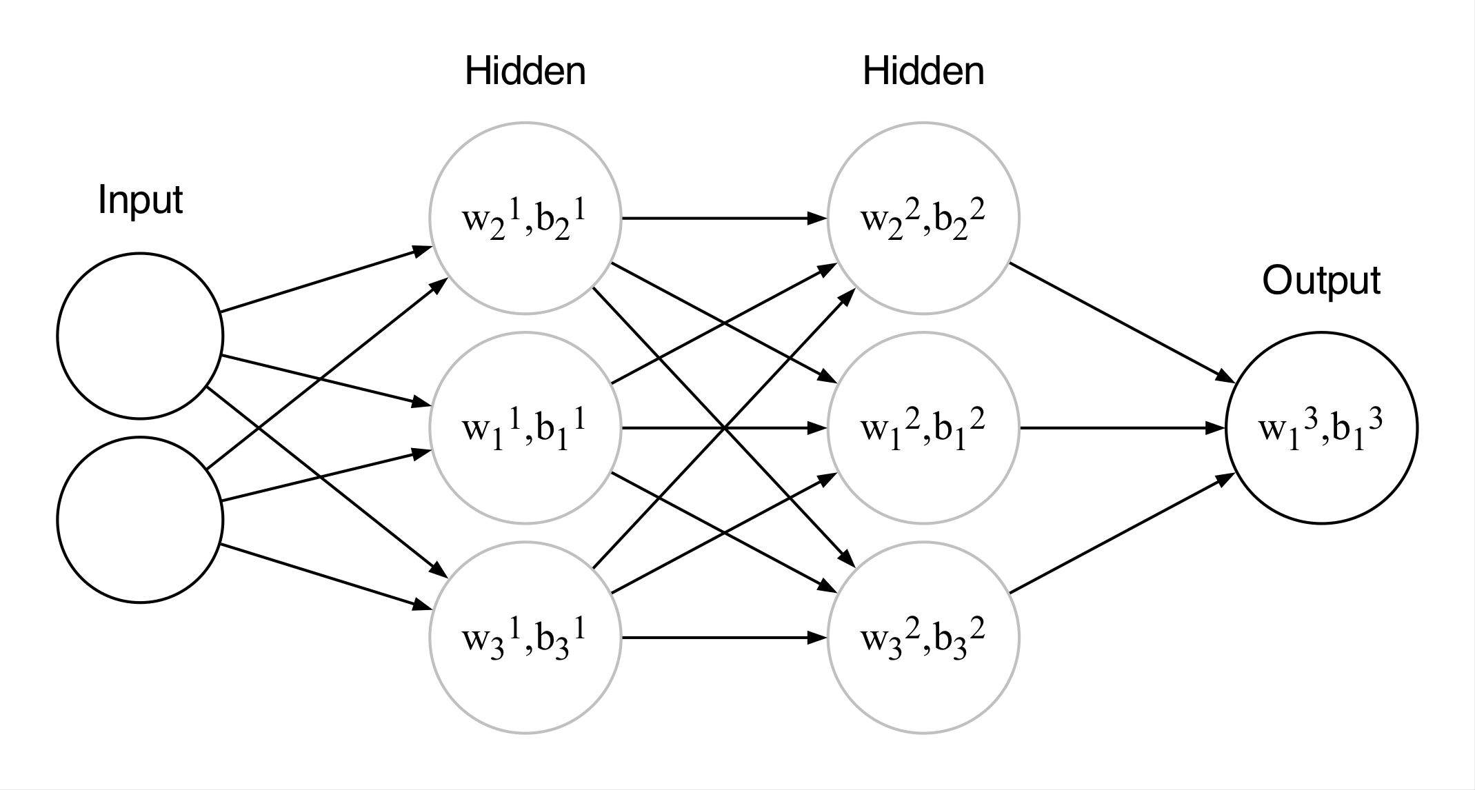
Three-layer neural network. $\mathbf w_i^l$ is the $i$th weight vector of the $l$th layer, and $\dim\left(\mathbf w_i^l\right) = \dim\left({\mathbf a_{l-1}}\right)$.
Row-Vector Notation
In contrast to scientific publications and textbooks, libraries like PyTorch or TensorFlow use right-multiplication notation:
\[f: \mathbb{R}^{M \times n} \to \mathbb{R}^{M \times m}, \quad f(\mathbf{X}) = \sigma(\mathbf{X}\mathbf{W}^\top + \mathbf{b}) \tag{5}\]where $\mathbf{W} \in \mathbb{R}^{m \times n}$, $\mathbf{b} \in \mathbb{R}^m$, and $M$ is the mini-batch size.
In this notation, the addition of the bias vector $\mathbf{b}$ to the matrix product $\mathbf{X}\mathbf{W}^\top$ is understood to be applied row-wise via broadcasting. Effectively, the bias is “stretched” across the mini-batch dimension so it can be added to each observation. Note that for a mini-batch size of $M=1$, this implementation is essentially the transpose of the textbook notation in Eq. \eqref{eq:multi-neurons}.
Why the difference?
- Batching Convention: In data science, rows represent observations and columns represent features. This matches standard dataset structures (CSVs, SQL).
- Hardware Efficiency: Modern GPUs use row-major storage. If data were stored as columns, the GPU would have to “jump” across memory addresses to fetch a single sample. Row-wise processing allows for memory coalescing, maximizing throughput.
Training and Optimization
The objective of training is to find the set of weights $\mathbf{W}$ and biases $\mathbf{b}$ that minimize the distance between the network output $\mathbf{o}$ and labels $\mathbf{y}$:
\[\hat{\mathbf{W}}, \hat{\mathbf{b}} = \arg\min_{\mathbf{W}, \mathbf{b}} \frac{1}{N} \sum_{i=1}^N C(\mathbf{W}, \mathbf{b}; \mathbf{x}_i, \mathbf{y}_i) \tag{6}\]Since calculating the inverse of the chained layers in Eq. \eqref{eq:multi-neurons} is virtually impossible, we must rely on numerical optimization. We use Stochastic Gradient Descent (SGD) to update parameters. The gradient $\nabla C$ indicates the direction of steepest increase; thus, we move in the opposite direction:
\[\mathbf{W}_t = \mathbf{W}_{t-1} - \eta \nabla_{\mathbf{W}} C, \quad \mathbf{b}_t = \mathbf{b}_{t-1} - \eta \nabla_{\mathbf{b}} C \tag{7}\]where the hyperparameter $\eta \in \mathbb{R}^+$ is the learning rate.
Note: While SGD remains a gold standard for training certain neural networks, adaptive optimizers like AdamW have emerged as the preferred choice for specific architectures.
The Role of Mini-Batches
In practice, calculating the cost over the entire dataset ($N$) is computationally prohibitive. Instead, we approximate the gradient using mini-batches of size $M < N$. Selecting the optimal $M$ is a balancing act between two competing forces:
- Stochasticity for Generalization: Because each mini-batch is a random sample, the resulting loss surface fluctuates slightly at every step. This “noise” is actually beneficial; it helps the optimizer escape sharp local minima and guides the network toward flat minima, which significantly improves the model’s ability to generalize to unseen data.
- Gradient Stability vs. Overfitting: Larger mini-batches provide a higher “gradient quality” by averaging out noise, leading to smoother and more stable updates. However, there is a point of diminishing returns: if $M$ is too large, the lack of stochastic pressure may cause the network to settle into poor minima or overfit on the training distribution.
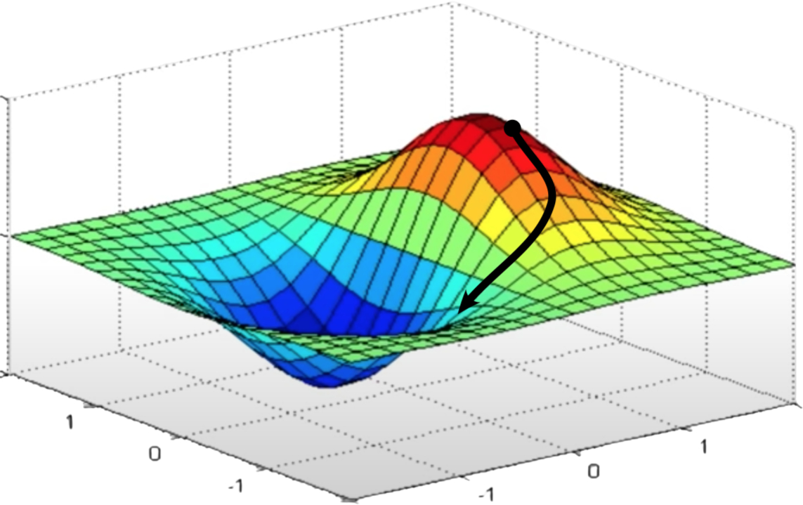
Loss surface at a given input $\mathbf x$.
Gradient Derivation
To calculate these gradients efficiently, we combine the chain rule with efficient matrix operators.
Prerequisites
In the following, we often use the gradient operator notation with respect to a matrix $\mathbf{M}$ or a vector $\mathbf{v}$ to denote the partial derivatives of the cost $C$:
\[(\nabla_{\mathbf{v}})_i = \frac{\partial C}{\partial v_i}, \quad (\nabla_{\mathbf{M}})_{ij} = \frac{\partial C}{\partial M_{ij}} \tag{8}\]Furthermore, we rely on the Multivariate Chain Rule. If a function $f$ depends on $x$ through several intermediate variables $g_i$, the total derivative is the sum of the partial derivatives along all paths:
\[\frac{\partial f}{\partial x} = \sum_{i} \frac{\partial f}{\partial g_i} \frac{\partial g_i}{\partial x} \tag{9}\]1. The Output Layer Error
Let $\mathbf{z}^l = \mathbf{W}^l \mathbf{a}^{l-1} + \mathbf{b}^l$. For the last layer $L$, the partial derivatives for a single weight and bias are:
\[\frac{\partial C}{\partial b_i^L} = \frac{\partial C}{\partial z_i^L} \frac{\partial z_i^L}{\partial b_i^L} = \frac{\partial C}{\partial z_i^L} \tag{10}\] \[\frac{\partial C}{\partial W_{ij}^L} = \frac{\partial C}{\partial z_i^L} \frac{\partial z_i^L}{\partial W_{ij}^L} = \frac{\partial C}{\partial z_i^L} a_j^{L-1} \tag{11}\]We define the error term $\delta_i^L := \frac{\partial C}{\partial z_i^L}$. In matrix form:
\[\boldsymbol{\delta}^L = \nabla_{\mathbf{a}^L} C \odot \sigma'(\mathbf{z}^L) \tag{BP1}\]2. Propagating Backward
For a hidden layer $l$, a change in $z_i^l$ affects the cost through all neurons $k$ in the next layer $l+1$. Summing these paths:
\[\delta_i^l := \frac{\partial C}{\partial z_i^l} = \left( \sum_k \frac{\partial C}{\partial z_k^{l+1}} \frac{\partial z_k^{l+1}}{\partial a_i^l} \right) \frac{\partial a_i^l}{\partial z_i^l} = \left( \sum_k \delta_k^{l+1} W_{ki}^{l+1} \right) \sigma'(z_i^l) \tag{12}\]Which gives the recursive matrix form:
\[\boldsymbol{\delta}^l = ((\mathbf{W}^{l+1})^\top \boldsymbol{\delta}^{l+1}) \odot \sigma'(\mathbf{z}^l) \tag{BP2}\]3. Parameter Gradients
Using the error terms, the final gradients for layer $l$ are:
\[\nabla_{\mathbf{b}^l} C = \boldsymbol{\delta}^l \tag{BP3}\] \[\nabla_{\mathbf{W}^l} C = \boldsymbol{\delta}^l (\mathbf{a}^{l-1})^\top \tag{BP4}\]Note on Batching: For a mini-batch size $M$, the total cost is $C_{\text{tot}} = \frac{1}{M}\sum C_i$. Consequently, the final parameter updates use the averaged gradients across the mini-batch.
Generalization
While FCNNs follow a rigid sequential structure, modern architectures like ResNets (with skip connections) or Transformers (with multi-head attention) are structured as Directed Acyclic Graphs (DAGs). In these networks, a single node’s output can be used by multiple downstream operations.
To compute gradients in a DAG, we move beyond “layers” and use Reverse-Mode Automatic Differentiation. This is the generalized engine powering PyTorch’s autograd and TensorFlow’s GradientTape.
The Generalized Chain Rule
If a variable $v_i$ influences the cost $C$ through multiple paths (successors), the total derivative is the sum of the derivatives along all those paths:
\[\frac{\partial C}{\partial v_i} = \sum_{j \in \text{Children}(i)} \frac{\partial C}{\partial v_j} \frac{\partial v_j}{\partial v_i} \tag{13}\]In this context, we often use the “bar” notation, where $\bar{v}_i = \frac{\partial C}{\partial v_i}$ represents the adjoint (or error signal) of $v_i$. This allows us to process any complex architecture by visiting nodes in reverse topological order.
Comparing Perspectives
| Sequential (FCNN) | Generalized (DAG) | |
|---|---|---|
| Perspective | Layers are treated as atomic blocks | Every operation (sum, mul, exp) is a node |
| Connectivity | Each layer has exactly one successor | A node can have any number of children |
| Error Signal | $\delta_i^l = \frac{\partial C}{\partial z_i^l}$ (Pre-activation error) | $\bar{v}_i = \frac{\partial C}{\partial v_i}$ (Node adjoint) |
| Gradient Flow | Pass error back through the weight matrix | Sum the error signals from all successor nodes |
This graph-based view explains how backpropagation handles modern complexities like residual connections—where the gradient simply “splits” and flows through both the skip path and the residual block—or weight sharing, where gradients from different parts of the graph are summed at the shared parameter node.
Conclusion
Backpropagation is a recursive application of the chain rule optimized through Dynamic Programming. It achieves a temporal complexity of $\mathcal{O}(P)$, where $P$ is the number of parameters, in a single backward pass. This linear efficiency is what allows us to train the massive models we see today.
References
- Nielsen, Michael A. Neural networks and deep learning. 2015.
- Goodfellow, Ian, et al. Deep learning. MIT press, 2016.